In this chapter we will discuss the general problems in control design. In the first section
the environment for design with its confinements and contradictory control aims will be
illustrated with a general blockscheme and an industrial plant. In the second section the
main control design strategies of today will shortly be characterized, their limitations and
benefits be indicated.

1.1 Control environment

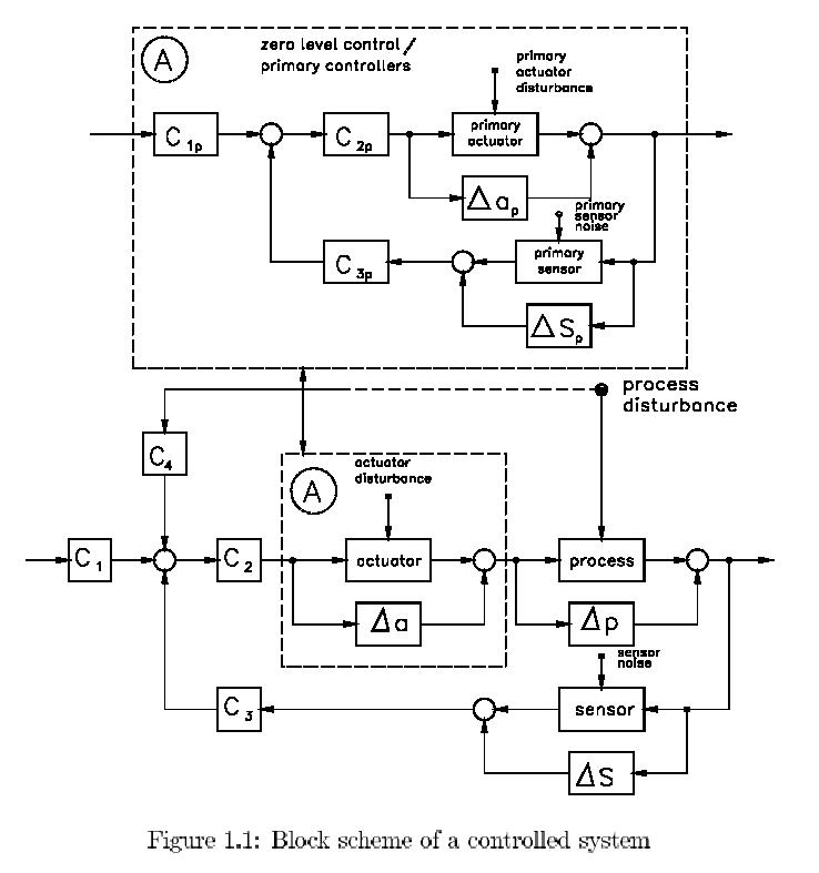
For facilitating the discussion consider a general and rather complete representation of
a controlled system in Fig. 1.1. The nominal model transfer function P of the plant to
be controlled is indicated by the block  “process". Because a model is always just an
approximation of the real world behavior P_t we have to cope with a model uncertainty
block ΔP that bypasses the model such that:
                          P_t = P + ΔP                                           (1.1)
During operation the actual output y of the plant is not only effected by controlled inputs
but also by process disturbances entering the process at various points. Generally these
disturbance effects are combined in a disturbance signal additive to the output.
     The actual inputs of the plant take the form of position, speed, force, torque, flow
of fluid, gas or heat, pressure and the kind, while the output of the controller generally
is a voltage from e.g. the DA-converter. In between we need an actuator that converts
the steering voltage into the proper quantity. This might be a pump, a (servo-)motor, a
valve, a burner, a heat exchanger, etc. and these all have in common that the effective
transfer is far from an ideal, static, linear function. Most often, (primary) controllers
have been applied to let the closed loop transfer of such actuators approximate a linear
transfer in a frequency band encompassing the dynamic behaviour of the ultimate plant to
be controlled. Consequently what we show on the level of the plant occurs as well on the
local level of the actuator which we have shown in Fig. 1.1 in the upper dashed block (A).
This actuator control is called `zero level control' by means of `primary controllers'. On the
level of the plant we just consider a (closed loop) actuator transfer model, its uncertainty
block _a and actuator disturbance analogously to the plant itself. In most textbooks the
actuator is not explicitly visualized but tacitly enclosed in the plant transfer.
     What has been said about the actuator applies to the sensor in a dual form. Actual
output quantities like position, speed, angle, rotation speed, fluid level, pressure, tem-
perature etc. is to be converted to a voltage in the proper range of the AD-converter.

Inevitably, the sensor transfer is not unity and we have to deal with transfer uncertainty
and sensor noise. Sometimes primary controllers and noise filters are used here as well to
improve the characteristics like in gyros, to control the rotation speed, or in measuring
servo systems.
     Finally we distinguish 4 blocks Ci that constitute the control:
     ・ C₁: a feedforward block that filters the reference signal, indicating the aimed level
              changes for the actual output.
     ・ C₂: a compensator block that adapts or corrects the actuator and plant transfer.
     ・ C₃: a feedback block that brings in the measured output signals.
     ・ C₄: a possible disturbance feedforward block. Sometimes disturbing quantities like
              environmental temperature, pressure, humidity, grid voltage fluctuations, light in-
              tensities etc. can be measured and used to improve the disturbance reduction by this
              control loop.
These control blocks C_i have to be designed such that the following goals and constraints
can be realized in some optimal form:

stability The closed loop system should be stable.
tracking The real output y should follow the reference signal ref.
disturbance rejection The output y should be free of the influences of the disturbances.
sensor noise rejection The noise introduced by the sensor should not affect output y.
avoidance of actuator saturation The actuator should not become saturated but has
          to operate as a linear transfer.
robustness If the real dynamics of the process change by an amount ΔP (and similarly
          for the actuator and the sensor), the performance of the system, i.e. all previous
          desiderata, should not deteriorate to an unacceptable level. (In explicit cases it may
          be that only stability is considered.)

It will be clear that all above desiderata can only be fulfilled to some extent. It will be
explained in chapter 2 how some put similar demands on the controllers C_i, while others
require contradictory actions, and as a result the final controller can only be a kind of a
compromise. To that purpose, it is important, that we can quantify the various aims and
consequently weight each claim against the others.
     As an example let us start with the disturbance reduction and tracking aim. In order
to reduce the effect of the disturbance and minimize the tracking error we can compare
the measured output with the reference by putting C₁ = 1 and C₃ = 1. Next a very
`large' C₂ can then in principle minimize the disturbance effects in the output to a very
low level. However, this very same high gained C₂ has very unpleasant side effects : the
stability is endangered, the actuator will saturate and the sensor noise will be introduced
and amplified to an unacceptable level. So these latter three constraints define the bound
for the best obtainable performance in the sense of disturbance reduction and tracking.
We can in principle relax the constraints by applying actuators with a broader range and
sensors with less noise. This implies higher powered and heavier actuators and higher
precision sensors that will certainly be more costly. So, eventually, the economic principle
defines the ultimate compromise that follows.
     Another example is that the robustness requirement weakens the other attainments,
because a performance should not only hold for a very specific process P, where the control
action can be tuned to very specifically, but also for deviating dynamics in ΔP. There is
no way to avoid ΔP considering the origins of it:

unmodelled dynamics The nominal model P will often be taken linear, time-invariant
          and of low order. As a consequence the real behaviour is necessarily approximated
          since real processes cannot be caught in those simple representations.
time variance Inevitably the real dynamics of physical processes change in time. They
          are susceptible to wear during aging (e.g. steel rollers), will be affected by pollution
          (e.g. catalysts) or undergo the influence of temperature (or pressure, humidity … )
          changes (e.g. day and night fluctuations in glass furnaces).
varying loads Dynamics can substantially change if the load is altered: the mass and
          the inertial moment of a robot arm is determined considerably by the load unless
          you are willing to pay for a very heavy robot that is also very costly in operation.
manufacturing variance A prototype process may be characterized very accurately,
          this is of no help if the variance over the production series is high. A low variance
          production can turn to be immensely costly if one thinks e.g. of a CD-player: in
          principle one can produce a drive with tolerances in the micrometer-domain but,
          thanks to control, we can suffice with less.
limited identification Even if the real process were linear and time-invariant, we still
          have to measure or identify its characteristics and this cannot be done without an
          error. Measuring equipment and identification methods, using finite data sets of
          limited sampling rate, will inevitably be suffering from inaccuracies.
actuators & sensors What has been said about the process can be attributed to actu-
          ators and sensors as well that are part of the controlled system. One might require
          a minimum level of performance (e.g. stability) of the controlled system in case of
          e.g. sensor failure or actuator degradation.

In Fig. 1.2 the effect of the robustness requirement is illustrated. In concedance to the

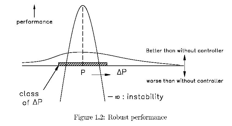
natural inclination to consider something better if it is higher, optimal performance is
a maximum here. So the vertical axis represents a performance aspect; a higher value
indicates a better performance. Positive values are representing improvements by the
control action and negative values denote a behaviour worse than without a controller.
For extreme values -∞, the system is unstable. In this super-simplified picture we let
the horizontal axis represent all possible process behaviours centered around the nominal
process P with a deviation ΔP living in the shaded slice. So this slice represents the class
of possible processes. If the controller is designed to perform well for just the nominal
process, it can really be fine-tuned to it, but for a small model error ΔP the performance
will soon deteriorate dramatically. We can improve this effect by robustifying the control
and indeed improve the performance for greater ΔP but unfortunately and inevitably at
the cost of the performance for the nominal model P. One will readily recognize this
effect in many technical designs (cars, bikes, tools, ... ), but also e.g. in natural evolution
(animals, organs, ... ).
     In above sketch of the environment for control design we have tacitly assumed that all
blocks have only one input signal and one output signal like in most of the conventional,
basic control textbooks. We then talk about SISO-systems (Single Input Single Output).
For the general plants, to be discussed, the relevant transfer may be multivariable resulting
in a MIMO (Multi Input Multi Output) transfer. In the multivariable case all above single
lines then represent vectors of signals. For example, in a CD-player the laser beam has to
be focussed on the track in the CD despite of the radial and vertical unbalance caused by
the rotation. Because the radial and vertical disturbance and control interact we really
deal with a MIMO-process. In stead of such a single product we would like to exemplify

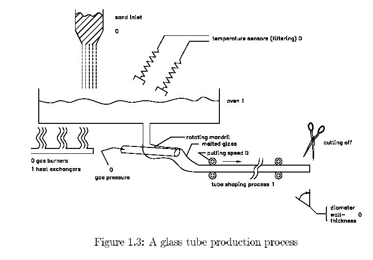
control design categories by means of a production plant as sketched in Fig.1.3. By this
production unit, glass tubes are manufactured for e.g. fluorescent lamps. Immediately two
subprocesses can be distinguished on level 1 where we reserved level zero for the implicit
actuator control. On the one hand we have the glass furnace where the raw material sand
is transformed into a melted glass stream of the proper viscosity. On the other hand we
have the tube shaping process where the glass flow is moulded to a glass tube.
     For the furnace, the control inputs are the sand inflow, the gas flow to the burners,
the pressure of the cooling air and the outputs are the melted glass outflow and its tem-
perature which directly determines its viscosity. Disturbances on the outputs are caused
by fluctuations in the composition of the raw material and the caloric value of the gas and
the air temperature.
     The shaping of the tube is realized by winching the steady glass flow on a rotating
mandrel under a certain tilting angle from which the glass drains into what is called a
`ham'. This ham is kept under a certain pressure by the gas that is pressed through the
hollow mandrel. The tube is then continuously pulled from the ham and transported under
slow rotation over a length of about 60 meters for cooling. At the end, the tube is cut into
pieces of proper length. The inputs of this shaping process are the mandrel gas pressure
and the pulling speed. The outputs are the diameter and wall thickness of the tube
measured at some distance from the ham because of the extreme heat. As disturbances
can be mentioned the variations of the glass flow and the viscosity (so the tracking errors of
the previous process), air temperature and pressure, effects of the rotation of the mandrel
and the pulling machine (e.g. eccentricity of the wheels and bearings).
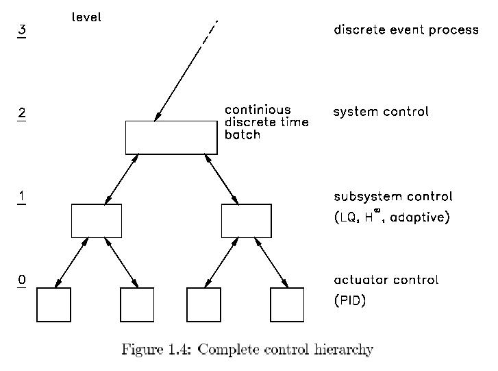
Let us explicitly discuss the control at several levels now, as hinted at before and
illustrated in Fig. 1.4:

     ・ level 0: At zero level the actuators and permanent conditioning processes are con-
        trolled, like: the actuators for the sand inlet , the gas pressure, the cooling air, the
        mandrel gas pressure, the pulling speed and the processes that keep the mandrel and
        the tube itself in constant rotation. This control is mostly done by the conventional
        PID-controllers or, in case of strong nonlinearities, by means of dedicated nonlinear

       control techniques.
     ・ level 1: At level one we distinguish the subprocesses with clear inputs and outputs
       that depend on each other, like here the furnace and the shaping process. Tradition-
       ally the control was done by operators but is gradually assisted or even taken over
       by MIMO-control techniques like LQG-control, adaptive control and robust control
       to be discussed in the next section.
     ・ level 2: On this level the interaction between the various subprocesses is kept under
       control by adapting the reference signals. In principle the same techniques can be
       used as for the previous level but on a much slower time scale.
     ・ level 3 : Here the inventory control of the raw material, the products in the form of
       categories of tubes, the gas supply, the costs of electricity is taken place. Completely
       different techniques are in use, like discrete event process control that will not be
       discussed here.
     ・ level 4 : After some time the furnace has to be rebuild because of degradation of
       the walls. Also the mandrel wears and the pulling machine needs servicing. This
       time scheduling and long term planning has time constants in the order of weeks to
       months.
     ・ level 5 : At an even lower pace runs the planning for the housing and product
       selection for the whole enterprise, where economic control is central.

     By means of above hierarchy of levels the problem of hierarchic control is easy to grasp.
The higher the level the lower the pace. Each lower level acts more or less as an all pass
process for the frequency band of its upper level. There is a command stream from above
that puts severe constraints on the lower level process control by means of the reference
signals that can thus be rather low frequent. The control at the higher levels is based upon
information from the lower level. But this lower level proceeds at a much higher rate so
that there is much too high an information density unnecessary for the higher level. An
appropriate information stream is therefore indispensable which is balanced between the
data overload and information insufficiency. Both can lead to low performance or even
instability.
     So the real environment of control design teaches us that we have to deal with multi-
variable systems, that control will be a compromise in the fulfillment of contradictory aims
and constraints, that control performance has to be robust for model perturbations and
that the systems might be embedded in an hierarchical structure.
     There is still another issue that becomes evident from the example of the glass tube
production line. In the start up situation it will be clear that we have to deal with a
substantially nonlinear process. The furnace has to be heated up from zero and special
techniques are necessary to pull the initial tube from the ham. A similar situation occurs
at the shut down procedure. Less pronounced, but nonetheless nonlinear, is the behaviour
in the change over trajectory where the production is changed from one diameter and wall
thickness to another set of these. The control of this change over is substantially different
from the control in a constant working point where indeed a linear model with a linear
controller could do the job. So the issue is how to deal with nonlinear plants. We list the
following approaches:

     ・ single linearisation. If the signals just show small excursions about some average
        value, the obvious solution is to linearise the plant in the proper equilibrium or
        working point. The nonlinear effects are then supposed to remain relatively small
        and can be treated as model perturbations or considered as disturbances. This
        way the linearised plant can be controlled by classical PID-controllers or, if better
        quantisised, by robust control techniques.
     ・ multiple linearisation. If the range is to big to be covered by a single lineari-
        sation, it can be partitioned into overlapping subranges for each of which a single
        linearisation can be developed. The overlapping is then necessary to switch from
        the one linearisation to the other. This switching should be taken very literal be-
        cause the model is changing and thus the necessary controller as well. So the one
        controller is switched o_ while the other is switched on. The problem then hides
        in the initial state of the controller that is switched on. It takes some time before
        the transient is died out or one has to `warm up' the controller before the switching
        which requires special techniques and puts constraints on the controller. On top of
        that, one has to make sure that the next moment the switching is not again reversed
        so that a kind of oscillation occurs. This is overcome by the mentioned overlap and
        by a properly defined switching hysteresis. Nevertheless, it appears to be difficult
        to realize a bumpless transition . As an alternative a "fuzzy" transition is proposed,
        where the output of the one controller is gradually diminished and overtaken by the
        output of the other controller. Consequently we have to deal with a weighted sum of
        both controllers in parallel which effect is hard to analyse for e.g. stability. Finally
        and again one has to compromise between a fine meshed partitioning for the best
        linearisation and a minimum number of transition `bumps'.
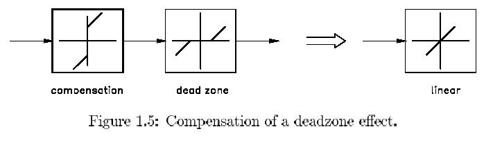
     ・ linearisation by compensation. If the nonlinearity is essentially nondynamic it
       can be compensated by the static complementary function. As an example the dead
       zone can be taken as illustrated in Fig. 1.5 where the complementary function is
       also shown. In this way one can e.g. compensate for the nonlinear valve character-
       istics, nonlinear transmission rates, friction characteristics and also nonlinearstatic
       measurements.

     ・ adaptive control In the case that the plant dynamics are linear over limited time
        horizon but that they change over the long run, adaptive control can be applied.
        During the time span that the dynamics can be supposed to be linear and time
        invariant, the transfer function is estimated and a proper controller tuned for this
        transfer. This estimation and tuning is then continued on-line so that slow change
        in time can be followed.
     ・ linearisation by feedback. Under certain complex conditions, that can be verified
        if the plant dynamics are not too complicated, the dynamics can be made linear
        by means of a nonlinear feedback. Not only for a limited range as for the single
        linearisation, but for the very range for which the nonlinear model holds true. It can
        only be applied if the model is very good and if sensor noise and disturbances can
        be neglected to a certain level. This can e.g. be true for mechanical systems like
        robots.
     ・ nonlinear control One can attack the nonlinear plants in their own nonlinear
        domain by dito controllers. Soon, if the plant is somewhat complex, this founders
        on the very complex computations.
     ・ `intelligent control'. As the previous approach suffered from the complexity of the
        analytical computations, it is often tried nowadays to find the nonlinear dynamic
        controller by optimization within a set of nonlinear, dynamic transfers. This set
        can be a neural network or a fuzzy logic based controller. The techniques will be
        discussed in later sections but the main problem is in the choice of the controller set
        and in the optimization: One never knows whether the set is big enough and the
        optimization can stop in a local extremum.
        If the nonlinearity has a `conditional' character expert systems can help. It will be
        clear that conventional PID controllers can do very little in case a sensor or actuator
        breaks down. However, an expert system can choose the proper strategy if it is well
        designed.