1.2.1 Classic control.
This category contains the conventional PID-controllers possibly implemented in a digital
system. The design of these controllers is based upon frequency domain descriptions like
the familiar Nyquist-, Bode-, Nichols-diagrams and root locus techniques. They cover
most control actions in level 0 for actuators to steer the proper pressure, temperature,
speed, flow etc. and as such they are responsible for about 80 to 90% of the control in
industry. Nevertheless, they also proved their value in level 1 systems provided that these
are SISO, e.g. the application in ship steering control.
For the tuning of these PID-controllers a rough, low order approximate model is suf-
ficient. In general, finer tuning can improve the performance but the majority of them
are operated largely at the safe side of the margin so that they are robust against plant
perturbations. Well known rule of the thumb criteria for the stability robustness are listed
as the (45°-)phase margin, the gain margin and the M-circles. The theory can be found
in many classic control textbooks.
strong aspects: easy to design, simple models suffice, robust, available as industrial
components
weak aspects: only for SISO, suboptimal

1.2.2 Nonlinear control.
In the previous section a list of possible strategies to attack nonlinear systems has been
given. The nonlinear control is designed on the basis of the nonlinear systems equations.
By means of
the variation calculus, the Hamiltonian and Pontryagin's maximum principle the solution
can analytically be computed resulting in a set of nonlinear differential (or difference)
equations with boundary conditions at both ends of the time period for which optimisation
is required. This TPBVP (two point boundary value problem) is still hard to solve and
computations soon become very complicated. Nevertheless, for simple systems it can
be well applied under the condition that the model is accurate and sensor noise and
disturbances are very small. On top of that, this approach provides lots of insight in
the behaviour of nonlinear processes and forms the basis for linear control design in time
domain like the LQG-control.
strong aspects: powerful analysis, direct optimal design
weak aspects: only possible for simple plants, not robust, accurate model necessary,
noise and perturbations should be negligible

1.2.3 LQG-control
Departing from the state space description some forty years ago a start was made to design
controllers in time domain for multivariable (MIMO) plants. It was soon discovered that,
as the states represent all memory of the plant, a simple static state feedback in the form
u = -Lx (see Fig.1.6) for linear plants could position the poles of the closed loop system
at will. That way, the dynamics of the closed loop system could theoretically be well
suited to reduce the disturbance h at the output y. In practice it turned out that the
range of the actuator put bounds on the ultimate performance. Nevertheless, by means
of a proper criterion a well balanced solution can easily be obtained. The main problem
lurked in the availability of all states where usually only the output y is measured. This
problem is overcome by exciting a model of the plant by the same input u so that an

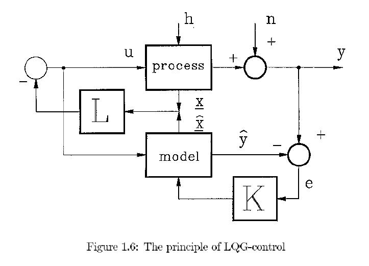
estimate ^x of the real state x (see Fig. 1.6) becomes available. This estimate then only
incorporates the effects of the input u and not the disturbance results of h which are only
apparent in y. A feedback loop of the difference between the actual and the model output
via a static gain K (the so called Kalman gain ) `simulates' the disturbance h for the
model which substantially improves the estimate ^x in particular for large values of K.
Unfortunately the measurement noise n limits this K because too large a Kalman gain
introduces too much measurement noise into the loop and thus into the output y. Again
by means of balanced criteria , optimal solutions can be obtained that take care for both
actuator saturation and sensor noise. So a well tuned control action will result in case an
accurate model of the plant is available. These technique has proved its usefulness e.g. in
space control where the dynamics are very accurately known. In industry this is quite the
opposite and robustness is hard to analyze and guarantee by this technique.
strong aspects: MIMO, clear analysis, easy design, fine tuned including saturation and
sensor noise
weak aspects: not robust, a very accurate model is indispensable

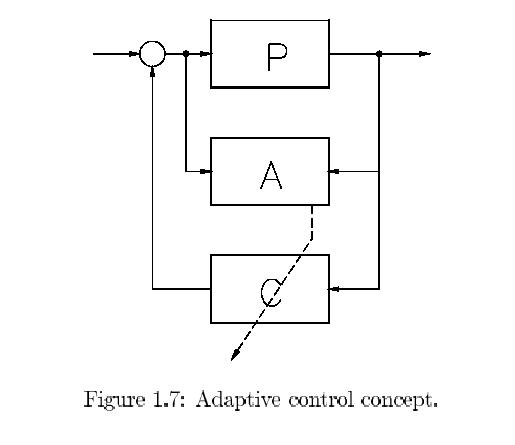
1.2.4 Adaptive control
If the dynamics of a plant are predominantly linear but change slowly in time adaptive
control can be applied. Fig.1.7 illustrates the principle. Let a controller C be designed by
some of the other linear systems control designs based upon the model of the plant. So
the design might be classic or LQG or pole placement or even H^∞ (to be discussed) but
such that given a model , a controller C can be computed and even better be corrected
(adapted) as soon as the model is updated. The updating of the model is executed by
an on line estimation algorithm that is fed by the inputs and the outputs of the real
process.
In order to estimate a sufficiently accurate model the on-line estimation algorithm needs a
data set of at least five times the effective length of the impulse response of the plant. So
.
updating can not take place faster than this period and the variation of the plant should
therefore be of an even slower rate. A second bottle neck might be the computational
speed available for the estimation and control design. So inevitably adaptation is slow
and the designed control should be `cautious' in order to preserve sufficient robustness
against model inaccuracy. A good introduction into adaptive control can be found in [1].
strong aspects: facilitates wide range control of slowly timevariant plants, many options
and variations possible
weak aspects: cautious because of robustness and thus rather slow, theory not yet well
established, only for slowly time variance.

1.2.5 MPC: Model Predictive Control
If the plant, to be controlled, is very complex, has many inputs and outputs, its model is
very weak and actuators are soon saturated, alternative control designs will fail as they
involve too many computations. This often occurs in (chemical) process industry. The
MPC can help as it combines approximate modeling and cautious control with modest
computational burden. This method is resembling the adaptive control. It also includes
on-line identification of a simple, low order model, possibly even zeroth order. It requires
only limited computation, because a prediction model can be used so that a simple equation
error criterion can be applied, leading to a one shot solution i.e. no iterations. Next, based
on this model, an LQG-control is designed. The penalty on the input and the modest claim
of reaching the reference level on a finite horizon of tens of samples results in a necessarily
cautious control which avoids actuator saturation. Only the first control sample is applied
after which the whole cycle of identification and LQG-control design is repeated for the
next time instance. This strategy improves robustness. More detailed information can be
found in [2] and [4].
strong aspects: enables control for complex, large scale plants with poor modeling
and limited actuators.
weak aspects: too cautious control with low performance for well modeled plant
of lower complexity.

1.2.6 Robust control.
The classic control is certainly `nonoptimal' as it is based on rough models and rule of the
thumb safety margins but, because of this, it yields robust controllers. The design is done
in frequency domain. LQG-design allows fine tuning of the controllers in time domain
but lacks necessarily robustness. It was not until the beginning of the eighties that an
intermediate solution emerged between these extremes in the form of the robust control
techniques. Essentially the classic control was given a sound mathematical fundament
for quantisation and balancing of all the control requirements as we have listed in the
previous section. By proper filters and norms the reference signals, the disturbances and
the measurement noise can be characterized. The control aims can likewise be weighted
mutually and the effect of model perturbations can be accurately brought into the problem
definition. In the next chapters the essential procedure for this will be introduced. By this
accurate characterization and weighting, it is possible to numerically define the wanted
balance between fine tuning and robustness at will. This can be done in frequency domain
yielding the so called H^∞-control, where the errors in performance are measured in energy
or power. In time domain the result is l₁-control where the peaks in the performance errors
are minimized. There is even a counterpart of LQG-control to be described in this context
by the name of H²-control. They all have in common that if the model perturbations can be
bounded in a clearly defined set, the final controller will guarantee stability and a minimum
level of performance for even the "worst case" model perturbation allowed. As it is worst
case robust, it must necessarily be very "pessimistic" so that rather cautious controllers
result. This "conservatism" is mainly caused by the rather crude characterization of
model errors. If the modeling error is quantified in more detail and thus more accurate a
refinement is possible and this culminated into the so called μ-analysis/synthesis.
strong aspects: robust control in the face of model errors
weak aspects: cautious control

1.2.7 Intelligent control.
Intelligent control is only a collective noun for controllers that at a remote superficial look
seem to take decisions. If the plant is in a certain state the controller takes a specific,
preprogrammed action. For instance the plant might tend to be overloaded so that pre-
cautions are taken to relax the load. Or a sensor and an actuator seem to have been
broken down so that the plant has to be kept in a steady, stable state until things have
been repaired. One can extent this to quantitative control. The larger an output becomes
the stronger an actuator is activated. In that way a simple proportional control can be
realized. As we can plit up the total ranges it is easy to create a nonlinear, static control.
If we also operate upon derivatives and integrals we thus have a potential to combine
switching operations with all kinds of nonlinear, dynamic control actions.
     Three categories and a combination belong to this intelligent control:
Expert systems Particularly `logic' control can be implemented in such a system that
consists of long series of conditional commands of the form: "if" ・・・ "then" ・・・ "else"
・・・ . In case that the condition is first checked followed by the proper command we
speak about `forward chaining'. The opposite can be applied as well where the last
command is executed until the condition prescribes another action. This is called
'backward chaining' and offers the advantage of higher speed. By internal feedback
a certain learn capacity can be created. It will be clear that these expert systems
are highly specialized and confined to a very restricted domain. In our application of
control (they are also frequently used for e.g. diagnosis) the conditional commands
are based upon the long experience of operators that used to control the specific
plant. Their experience is translated into the expert system and at best it can thus
come up to the level of the operators if translation were perfect. In practice this
appears to be the Achilles' heel because human beings react on far more things
than they are aware of and what can be translated into the confined domain of
operation.
Fuzzy logic controllers The classical logic, knowing only two levels `true' and `false',
can be refined by admitting expressions like `more true' and `less false'. Famous
examples are categories indicated by relative adjectives young, old, bald, fat, tall,
warm, cold etc. contrary to the (more) crisp adjectives alive, dead, pregnant, male,
female etc. Not only is this obvious in daily live but also in technical plants it is
evident. In fact all signals are not in a binary space but on a continuous scale. Also
`fuzzy' observations like \the rudder does not function well", "there is a smell of
burning so something might be overheated" or commands like "be cautious", "a fast
reaction is wanted" can be cast into the domain of fuzzy logic. Without entering
into details here (see later in chapter 4.7) experience and straightforward guessing
can be moulded in a fuzzy set logic that finally boils down to a static, nonlinear
transfer between a set of measurements and a set of control lines. If this does
not function satisfactorily corrections can be made until sufficient performance is
obtained. The weak point is again the translation phase into the fuzzy logic. The
number of characterizing sets is for instance 7 in the following example of a signal
characterization: `very negative', `negative', `small negative', `zero', `small positive',
`positive', `very positive'. The greater the number of sets per signal the more refined
the nonlinear function can be but the more complicated the controller becomes
leading to long processing times. But even more important is the fact that many
implementations of the fuzzy logic are possible and the last operation, to arrive at
real signals from set `memberships', the so called "defuzzification", is also far from
unique. This introduces quite an amount of arbitrariness into the implementation
and only trial and error can reduce this effect.
Neural network control Initially, in the field of neural networks the biological neurons
were simply modeled as switching elements reacting on the weighted sum value of a
set of inputs. These `neurons' are then combined in parallel in a layer and in series in
consecutive layers. They were then trained by varying the weights until the proper
output was switched on if a certain input pattern was applied. In this way they
proved to be useful as pattern recognition tools.
Soon the pure switching function (step function) in the neuron was replaced by
a smooth function (a sigmoid function like the arctangent) to cope with gradual
phenomena like the transition from classic logic to fuzzy logic. In this way we
again have a nonlinear, static function where the tunable resolution depends on
the number of neurons and the number of weights. The next phase is the training
where the weights are changed until a wanted behaviour is obtained, measured in
some scalar criterion. By feeding back delayed samples of the output of the neural
net to its inputs a dynamic discrete time transfer can be created that can function
as a model or a controller of a plant. By training, the modelling or controlling
performance can then tried to be optimized. This is the troublesome stage, because
the total system behaves as a black box where one cannot analyze the effects of the
various weights at all. In linear system identification we speak about a black box
if we try to fit the behaviour of a linear, dynamic transfer where the parameters
are just the coefficients of linear difference equations. The capacity or complexity
of the black box is then expressed in the number of parameters directly determined
by the number of states. For these nonlinear neural network based transfers the
extra complication is in the characterization of the nonlinearity by the number of
neurons. One could say that one is trying to train a "black squared" box with all the
problemsarising with it. How many neurons for describing the nonlinearity and how
many internal feedback loops for describing the number of states should one allow in
order to let the system be complex enough for the task it should execute? Moreover,
parsimony is required because very soon the number of parameters explodes that
tackles the training as unacceptable computational power and time is necessary
and optimization gets stuck in local extrema. Here the potential power conflicts
with computational requirements. Also biological evolution took its time and every
student would like to have more time available for his study.
Neuro-fuzzy control It is easy to recognize that fuzzy logic and neural nets are just
doing similar things on a different basis. They both approximate general, static
, nonlinear functions by combination of smaller components. Also central basis
functions do the same thing with other components and it is not difficult to design
your own building blocks and composition for still another `new' method. The
analogy goes even further when a so called `one hidden layer neural net' is compared
with a fuzzy logic transfer. The weights appear to be the memberships, the neural
functions to be the membership functions and so on. Effectively the two methods
are then congruent apart from different names. So it is then natural to melt them
together in the field of the neuro-fuzzy controllers.
strong aspects: A great potential to combine quantitative operations with switching
based on logic.
weak aspects: translation of experience imperfect, arbitrariness and black box, lack of
analysis, problems in optimization
This ends the superficial survey of methods. In the next chapters more attention will be
paid to the fundamental, internal conflicts in control design and the relevance of the model
for and in the controller will be stressed by the internal model control. In the last chapter
some control design methods will be treated in more detail.
 

Bibliography
[1] K.J._Astrom and B.Wittenmark, "Adaptive Control", Addison-Wesley, second edition
1995.
[2] D.W.Clarke, C.Mohtadi and P.S.Tu_s, "Generalized Predictive Control", parts 1 and
2, Automatica, 23, 137-160.
[3] A. Isidori,"Nonlinear Control Systems: an Introduction", Lecture Notes in Control
and Information Sciences 72, Springer Verlag 1985.
[4] M. Morari and E. Za_riou, "Robust Process Control", Prentice Hall 1989.
[5] H. Nijmeijer and A.J.van der Schaft,"Nonlinear Dynamical Control Systems", Springer
Verlag 1990.