In this chapter we will list and analyze the various goals of control in more detail. The
relevant transfer functions will be defined and named and it will be shown how some
groups of control aims are in conflict with each other. To start with we reconsider the
blockscheme of a simple situation in Fig. 2.1. Notice that we have made the sensor noise

explicit in η. In principle the sensor itself has a transfer function unequal to 1 so that this
should be inserted as an extra block in the feedback just before the sensor noise addition.
However, a good quality sensor has a at frequency response for a much broader band than
the process transfer. In that case the sensor transfer may be neglected. Only in case the
sensortransfer is not sufficiently broadbanded (easier to manufacture and thus cheaper)
a proper block has to be inserted . In general one will avoid this because the ultimate
control performance highly depends on the quality of measurement: the resolution of the
sensor puts an upper limit to the accuracy of the output control as will be shown.
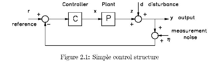
     The process or plant (the word "system" is more or less reserved for the total, controlled
structure) incorporates the actuator. The same remarks as made for the sensor hold for
the actuator. In general the actuator will be made sufficiently broadbanded by proper
control loops and all possibly remaining defects are supposed to be represented in transfer
P.  Actuator disturbances are combined with the output disturbance d by computing or
rather estimating its effect at the output. Therefor one should know the real plant transfer
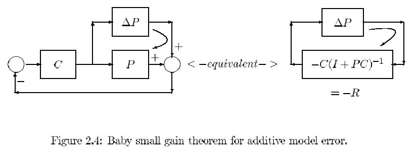
Pt consisting of the nominal model transfer P plus the possible, additive model error ΔP.
As only the nominal model P and some upper bound for the model error ΔP is known, it
is clear that only upper bounds for the equivalent of actuator disturbances in the output
disturbances d can be established. The effects of model errors (or system perturbations) is
not yet made explicit in Fig. 2.1 but will be discussed later in the analysis of robustness.
     Next we will elaborate on various common control constraints and aims. The con-
straints can be listed as stability, robust stability and avoidance of actuator saturation.
Within the freedom, left by these constraints, one wants to optimize, in a weighted balance,
aims like disturbance reduction and good tracking without introducing too much effects of
the sensor noise and keeping this total performance on a sufficient level in the face of the
system perturbations, i.e. performance robustness against model errors.  In detail:
     Stability. Unless one is designing oscillators or systems in transition , the closed loop
system is required to be stable. This can be obtained by claiming that nowhere in the
closed loop system some finite disturbance can cause other signals in the loop to grow to
infinity: the so-called BIBO-stability from Bounded Input to Bounded Output. Ergo all
corresponding transfers have to be checked on possible unstable poles. So certainly the
straight transfer between the reference input r and the output y given by :
                   y = PC(I + PC)^-1r                                             (2.1)
But this alone is not sufficient as, in the computation of this transfer, possibly unstable
poles may vanish in a pole-zero cancellation. Another possible input position of stray
signals can be found at the actual input of the plant additive to what is indicated as x
(think e.g. of drift of integrators). Let us define it by d_x. Then also the transfer of d_x to
say y has to be checked for stability which transfer is given by:
                  y = (I + PC)^-1Pd_x = P(I + CP)^-1d_x                      (2.2)
Consequently for this simple scheme we can distinguish four different transfers from r and
d_x to y and x, because a closer look soon reveals that inputs d and η are equivalent to r
and outputs z and u are equivalent to y.
     Disturbance reduction. Without feedback the disturbance d is fully present in the
real output y. By means of the feedback, the effect of the disturbance can be influenced
and at least be reduced in some frequency band. The closed loop effect can be easily
computed as read from:

The underbraced expression represents the Sensitivity S of the output to the disturbance
thus defined by:
                   S = (I + PC)^-1                                                  (2.4)
If we want to decrease the effect of the disturbance d on the output y we thus have to
choose controller C such that the sensitivity S is small in the frequency band where d has
most of its power or where the disturbance is most “disturbing".
     Tracking. Especially for servo controllers but in fact for all systems where a reference
signal is involved ,there is the aim of letting the output track the reference signal with a
small error at least in some tracking band. Let us define the tracking error e in our simple
system by:

Note that e is the real tracking error and not the measured tracking error observed as
signal u in Fig. 2.1, because the last one incorporates the effect of the measurement
noise substantially differently. In equation 2.5 we recognize ( underbraced) the sensitivity
as relating the tracking error to both the disturbance and the reference signal r. It is
therefore also called awkwardly the “inverse return difference operator". Whatever the
name, it is clear that we have to keep S small in both the disturbance and the tracking
band.
     Sensor noise avoidance. Without any feedback it is clear that the sensor noise will
not have any influence on the real output y. On the other hand the greater the feedback the
greater its effect in disrupting the output. So we have to watch that in our enthusiasm
to decrease the sensitivity, we are not introducing too much sensor noise effects. This
actually reminiscences to the optimal Kalman gain. As the reference r is a completely
independent signal, just compared with y in e, we may as well study the effect on the
tracking error e in equation 2.5. The coefficient (relevant transfer) of η is then given by:
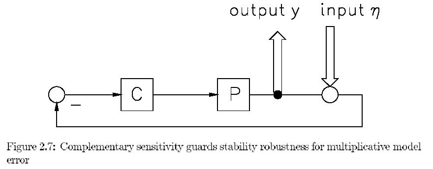
               T = PC(I + PC)^-1                                                       (2.6)
and denoted as the complementary sensitivity T. This name is induced by the following
simple relation that can easily be verified:
               S + T = I                                                                   (2.7)
and for SISO (Single Input Single Output) systems this turns into:
               S + T = 1                                                                 (2.8)
This relation has a crucial and detrimental influence on the ultimate performance of the
total control system! If we want to choose S very close to zero for reasons of disturbance
and tracking we are necessarily left with a T close to 1 which introduces the full sensor
noise in the output and vice versa. Ergo optimality will be some compromise and the
more because, as we will see, some aims relate to S and others to T.
     Actuator saturation avoidance. The input signal of the actuator is indicated by x
in Fig.2.1 because the actuator was thought to be incorporated into the plant transfer P.
This signal x should be restricted to the input range of the actuator to avoid saturation.
Its relation to all exogenous inputs is simply derived as:

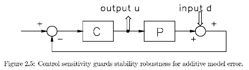
The relevant (underbraced) transfer is named control sensitivity for obvious reasons and
symbolized by R thus:
                R = C(I + PC)_1                                                         (2.10)
In order to keep x small enough we have to make sure that the control sensitivity R is small
in the bands of r, η and d. Of course with proper relative weightings and “small" still to
be defined. Notice also that R is very similar to T apart from the extra multiplication by
P in T. We will interpret later that this P then functions as a weighting that cannot be
influenced by C as P is fixed . So R can be seen as a weighted T and as such the actuator
saturation claim opposes the other aims related to S.
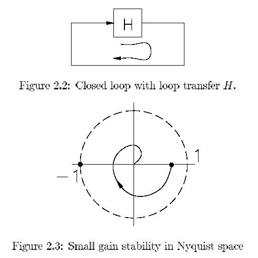
     Robust stability. The whole concept is based on the so-called small gain theorem
which trivially applies to the situation sketched in Fig. 2.2 . The stable transfer H repre-
sents the total looptransfer in a closed loop. If we require that the modulus (amplitude)
of H is less than 1 for all frequencies it is clear from Fig. 2.3 that the polar curve cannot
encompass the point -1 and thus we know from the Nyquist criterion that the loop will
always constitute a stable system. So stability is guaranteed as long as:


“Sup" stands for supremum which effectively indicates the maximum. (Only in case that
the supremum is approached at within any small distance but never really reached it is
not allowed to speak of a maximum.) Notice that we have used no information concerning
the phase angle which is typically H^∞. In above formula we get the first taste of H^∞ by
the simultaneous definition of the infinity norm indicated by ||・||_∞.
     All together, these conditions may seem somewhat exaggerated, because transfers, less
than one, are not so common. The actual application is therefore somewhat “nested" and
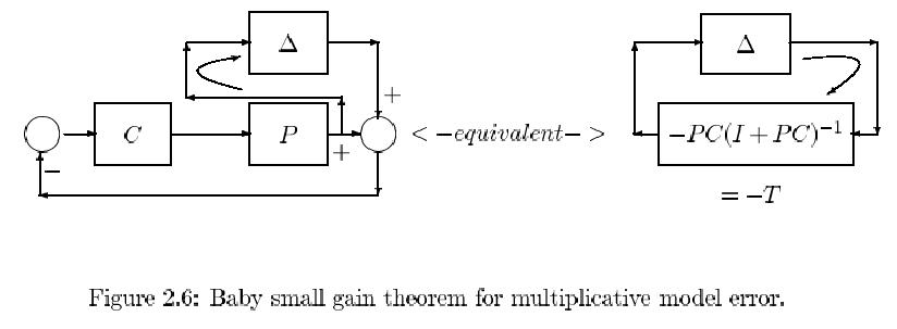
very depictively indicated as “the baby small gain theorem" illustrated in Fig. 2.4. In the

upper blockscheme all relevant elements of Fig. 2.1 have been displayed in case we have
to deal with an additive model error ΔP. We now consider the “baby" loop as indicated
containing ΔP explicitly. The lower transfer between the output and the input of ΔP,
as once again illustrated in Fig. 2.5, can be evaluated and happens to be equal to the
control sensitivity R as shown in the lower blockscheme. (Actually, we get a minus sign
that can be joined to ΔP. Because we only consider absolute values in the small gain
theorem, this minus sign is irrelevant: it just causes a phase shift of 180° which leaves
the conditions unaltered.) Now it is easy to apply the small gain theorem to the total

looptransfer H = RΔP. The infinity norm appears to obey Schwartz inequality so that
we may write:
         || RΔP||_∞ ≦ |R||_∞ ||ΔP||_∞                                       (2.12)
Ergo, if we can guarantee that :
          || ΔP||_∞ ≦  1/α                                                     (2.13)
a sufficient condition for stability is:
            || R||_∞ ≦  α                                                          (2.14)
If all we require from ΔP is stated in equation 2.12 then it is easy to prove that the
condition on R is also a necessary condition. Still this is a rather crude condition but it
can be refined by weighting over the frequency axis. Once again from Fig.2.5 we recognize
that the robustness stability constraint effectively limits the feedback from the point, where
both the disturbance and the output of the model error block ΔP enter, and the input of
the plant such that the looptransfer is less than one. The smaller the error bound α the
greater the feedback bound 1/α can be and vice versa!
We so analyzed the effect of additive model error ΔP. Similarly we can study the
effect of multiplicative error which is very easy if we take:
          P_true = P +ΔP = (I +Δ)P                                     (2.15)
where obviously Δ is the bounded multiplicative model error. (Together with P it evidently
constitutes the additive model error ΔP.) In similar blockschemes we now get Figs. 2.6
and 2.7. The “baby"loop now contains Δ explicitly and we notice that transfer P is
 

somewhat “displaced". The result is that Δ sees itself fed back by the complementary

sensitivity T. (Again by -T but the sign (phase) is irrelevant !) (The P has, so to speak,
been taken out ofΔP and adjoined to R yielding T.) If we require that:
           || Δ||_∞ ≦  1/β                                              (2.16)
the robust stability follows from:
           || TΔ||_∞ ≦ || Ｔ ||_∞ ||Δ||_∞ ≦  1                     (2.17)
yielding as final condition:
              || T ||_∞ ≦  β                                              (2.18)
Again proper weighting may refine the condition.
     Performance robustness. Till now all aims could be grouped around either the
sensitivity S or the complementary sensitivity T. Once we have optimized some balanced
criterion in both S and T and thus obtained a nominal performance, we wish that this
performance is kept more or less , irrespectively of the inevitable model errors. Conse-
quently performance robustness requires that that S and T change only slightly if P is
close to the true transfer P_t. We can analyze the relative errors in these quantities for
SISO plants:

     S_t - S       ( 1 + P_tC)^-1 - ( 1 + PC)^-1      1 + PC - 1 - P_tC       ΔP      PC
    ------- = ------------------------ = ---------------- = - --- ・ ------- = - ΔT
       S_t                   ( 1 + P_tC)^-1                       1 + PC                P      1 + PC

and :

     T_t - T      P_tC( 1 + P_tC)^-1 - PC( 1 + PC)^-1      P_tC - PC         ΔP    P        1
    ------- = ---------------------------- = ------------ = - --- ・ -- ・ ------- ��ΔS
       T_t                      P_tC( 1 + P_tC)^-1               P_tC(1 + PC)        P     P_t     1 + PC

As a result we note that in order to keep the relative change in S small we have to take
the product of Δ and T small. The smaller the error bound is, the greater a T can we
afford and vice versa. But what is astonishingly is that the smaller S is and consequently
the greater the complement T is (see equation 2.7), the less robust is this performance
measured in S. The same story holds for the performance measured in T where the
robustness depends on the complement S. This explains the remark in chapter 4 that
increase of performance for a particular nominal model P decreases its robustness for
model errors. So also in this respect the controller will have to be a compromise!

2.1 Summary

We can distinguish two competitive groups because S+T = I. One group centered around
the sensitivity that requires the controller C to be such that S is “small" and can be listed
as:
  ・ disturbance rejection
  ・ tracking
  ・ robustness of T
The second group centers around the complementary sensitivity and requires the controller
C to minimize T:
  ・ avoidance of sensor noise
  ・ avoidance of actuator saturation
  ・ stability robustness
  ・ robustness of S
If we were dealing with real numbers only, the choice would be very easy and limited.
Remembering that
           S = (I + PC)^-1                              (2.23)
           T = PC(I + PC)^-1                           (2.24)
a large C would imply a small S but T ≒ I while a small C would yield a small T and
S ≒ I. Besides, for no feedback, i.e. C = 0,  necessarily T → 0 and S → I. This is
also true for very large ω when all physical processes will have a zero transfer (PC → 0).
So ultimately for very high frequencies, the tracking error and the disturbance effect is
inevitably 100%.
This may give some rough ideas of the effect of C but the real impact is more difficult
as:
  ・ We deal with complex numbers .
  ・ The transfer may be multivariable and thus we encounter matrices.
  ・ The crucial quantities S and T involve matrix inversions (I + PC)^-1
  ・ The controller C may only be chosen from the set of stabilizing controllers.
It happens that we can circumvent the last two problems, in particular when we are dealing
with a stable transfer P. This can be done by means of the internal model control concept
as shown in the next chapter.