model structure is shown. The difference actually is the nominal model which is fed by the
In the internal model control the controller explicitly
contains the nominal model of the
process and it appears that in this structure it is easy
to denote the set of all stabiliz-
ing controllers. Furthermore the sensitivity and the
complementary sensitivity take very
simple forms expressed in process and controller transfer
without inversions. A severe
condition for application is that the process itself
is a stable one.
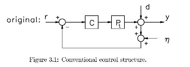
In Fig. 3.1 we repeat the familiar conventional structure
while in Fig. 3.2 the internal
model structure is shown. The difference actually is
the nominal model which is fed by the
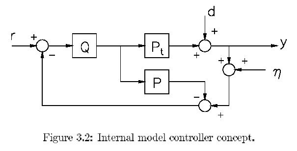
same input as the true process, while only the difference
of the measured and simulated
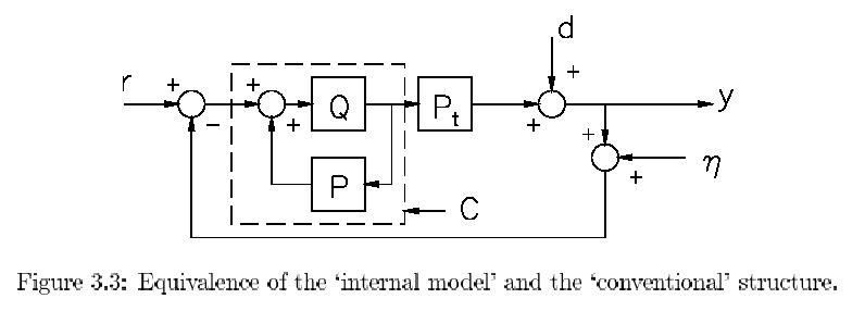
output is fed back. Of course it is allowed to subtract
the simulated output from the
feedback loop after the entrance of the reference yielding
the structure of Fig. 3.3. The
similarity with the conventional structure is then obvious,
where we identify the dashed
block as the conventional controller C. So it easy to
relate C and the internal model
control block Q as:
C = Q(1 - PQ)-1 (3.1)
and from this we get:
C - CPQ = Q (3.2)
so that reversely:
Q = (I + CP)-1C = C(I + PC)-1 = R (3.3)
Remarkably the Q equals the previously encountered control
sensitivity R ! The reason
behind this becomes clear if we consider the situation
that the nominal model P exactly
equals the true process Pt. As outlined before we have
no other choice than taking P = Pt
for the synthesis and analysis of the controller. Refinement
can only occur by using the
information about the model error ΔP that will be done
later. If then P = Pt, it is
obvious from Fig. 3.2 that only the disturbance d and
the measurement noise η are fed
back because the outputs of P and Pt are equal. Also
the condition of stability of P
is then trivial because there is no way to correct for
ever increasing but equal outputs
of P and Pt (due to instability) by feedback. Since only
d and η are fed back we may
draw the equivalent as in Fig. 3.4. So effectively there
seems to be no feedback in this
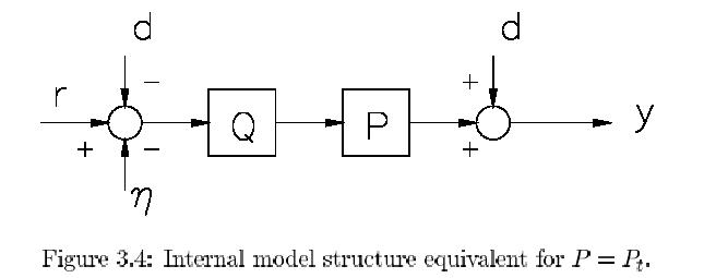
structure and the complete system is stable iff (i.e.
if and only if) transfer Q = R is stable
because P was already stable by condition. This is very
revealing as we now simply have
the complete set of all controllers that stabilize P
! We only need to search for proper
stabilizing controllers C by studying the stable transfers
Q. Furthermore, as there is no
actual feedback in Fig.3.4 the sensitivity and the complementary
sensitivity contain no
inversions but take so-called affine expressions in the
transfer Q easily derived as:
T = PR = PQ
S = 1 - T = 1 - PQ (3.4)
Extreme designs are now immediately clear:
・ minimal complementary sensitivity
T:
T = 0 → S = I → Q = 0 → C = 0 (3.5)
there is obviously
neither feedback nor control causing:
- no measurement influence (T=0)
- no actuator saturation (R=Q=0)
- 100% disturbance in output (S=I)
- 100% tracking error (S = I)
- stability (Pt was stable)
- robust stability (R=Q=0 and T=0)
- robust S (T=0), but this \performance" can hardly be worse.
・ minimal sensitivity S:
S = 0 → T = I → Q = P-1 → C = 1 (3.6)
if at least
P-1 exists and is stable, we get infinite feedback causing:
- all disturbance is eliminated from the output (S = 0)
- y tracks r exactly (S=0)
- y fully contaminated by measurement noise (T = I)
- stability only in case Q = P-1 is stable
- very likely actuator saturation (Q = R will tend to infinity)
- questionable robust stability (Q = R will tend to infinity)
- robust T (S = 0), but this “performance" can hardly be worse too.
Once again it is clear that a good control should be
a well designed compromise between
the indicated extremes. What is left is to analyze the
possibility of the above last sketched
extreme where we needed that PQ = I and Q is stable.
It is obvious that the solution could be Q = P-1
if P is square and invertible and
the inverse itself is stable. If P is wide (more inputs
than outputs) the pseudo inverse
would suffice under the condition of stability. If P
is tall (less inputs than outputs) there
is no solution though. Nevertheless the problem is more
severe, because we can show that,
even for SISO systems, the proposed solution yielding
infinite feedback is not feasible for
realistic, physical processes.
For a SISO process ,where P
becomes a scalar transfer, inversion of P turns poles into
zeros and vice versa. Let us take a simple example:
s - b
s + a
P = ----- , a .> 0, b > 0, → P-1 = -----
(3.7)
s + a
s - b
where the corresponding pole/zero-plots are shown in Fig.
3.5. It is clear that the original
zeros of P have to live in the open stable left halfplane
because they turn into the poles of
P-1 that should be stable. Ergo, the given
example, where this is not true, is not allowed.
Processes which have zeros in the closed right half plane,
named nonminimum phase, thus
cause problems in obtaining a good performance in the
sense of a small S.
In fact poles and zeros in the
open left half plane can easily be compensated for by Q.
Also the poles in the closed right halfplane cause no
real problems as the rootloci from

them in a feedback can be \drawn" over to the left plane
in a feedback by putting zeros
there in the controller. The real problems are due to
the nonminimum phase zeros i.e. the
zeros in the closed right half plane as we will analyze
further. But before doing so we have
to state that in fact all physical plants suffer more
or less from this negative property.
In order to analyze this further
we need some extra notion about the numbers of
poles and zeros, their definition and considerations
for realistic, physical processes. Let
np denote the number of poles and similarly nz the number
of zeros in a conventionally
transferfunction where denominator and numerator are
factorized. We can then distinguish
the following categories by the attributes:
proper if np ≧nz
biproper if np = nz
strictly proper if np > nz
nonproper if np < nz
Any physical process should be proper because nonproperness would involve:
lim P(jω) = ∞
(3.8)
ω→∞
so that the process would effectively have poles at infinity,
would have an infinitely large
transfer at infinity and would certainly start oscillating
at frequencyω= ∞. On the other
hand a real process can neither be biproper as it then
should still have a finite transfer for
ω= ∞ and at that frequency the transfer is necessarily
zero. Consequently any physical
process is by nature strictly proper. But this implies
that :
lim P(jω) = 0
(3.9)
ω→∞
and thus P has effectively (at least) one zero at infinity
which is in the closed right half
space! Take for example:
K
s + a
P = ---- , a > 0, → P-1 = ----
(3.10)
s + a
K
The disturbing fact about nonminimum phase zeros can now
be illustrated with the use
of the so-called Maximum Modulus Principle which claims:
∀H ∈ H∞ : || H ||∞ ≧ | H(s) |s∈C+ (3.11)
It says that for all stable transfers H (i.e. no poles
in the right half plane denoted
by (C+) the maximum modulus on the imaginary axis is
always greater than or equal
to the maximum modulus in the right halfplane. We will
not prove this but facilitate
its acceptance by the following concept. Imagine that
the modulus of a stable transfer
function of s is represented by a rubber sheet above
the s-plane. Zeros will then pinpoint
the sheet to the zero, bottom level while poles will
act as infinitely high spikes lifting the
sheet. Because of the strictly properness of the transfer,
there is a zero at infinity, so that
in whatever direction we travel, ultimately the sheet
will come to the bottom. Because of
stability there are no poles and thus spikes in the right
half plane. It is obvious that such
a rubber landscape with mountains exclusively in the
left halfplane will gets its heights
in the right half plane only because of the mountains
in the left half plane. If we cut it
precisely at the imaginary axis we will notice only valleys
at the right hand side. It is
always going down at the right side and this is exactly
what the principle tells.
We are now in the position to
apply the maximum modulus principle to the sensitivity
function S of a nonminimum phase SISO process P:

where zn (∈C+) is any nonminimum phase zero of P. As
a consequence we have to accept
that for some ωthe sensitivity will be greater than
or equal to 1. For that frequency
the disturbance and the tracking errors will thus be
minimally 100%! So for some band
we will get disturbance amplification if we want to decrease
it by feedback in some other
(mostly lower) band. That seems to be the price. And
reminding the rubber landscape
it is clear that this band, where S ≦ 1, is the more
low frequent the closer the troubling
zero is to the origin of the s-plane! By proper weighting
over the frequency axis we can
still optimize a solution.
Summary. It has been
shown that internal model control can greatly facilitate the
design procedure of controllers. It only holds, though,
for stable processes and the general-
ization to unstable systems is part of the robust control
theory. Limitations of control are
recognized in the effects of nonminimum phase zeros of
the plant and in fact all physical
plant suffer from these at least at infinity.